EFFECTS OF SEVERE ICING CONDITIONS ON AERODYNAMIC PERFORMANCE OF CESSNA 152 AIRCRAFT

ABSTRACT

The accretion of ice on an aircraft is dangerous to flight safety. Icing on a wing of an aircraft can significantly reduce the aerodynamic performance. There are different types of icing conditions resulting in different ice accretions. Hence, evaluation of the process and outcomes of ice accretion is vital to ensure safety. In this project, the adverse effects of ice accretion on aircraft are studied. The icing effects are examined using experimental, numerical and theoretical methods. A brief comparison between the results, achieved by comparing the three methods, of this project with the published data, suggest that the findings of this study are valid and useful.

TABLE OF CONTENTS

DECLARATION STATEMENT

ABSTRACT

TABLE OF CONTENTS

LIST OF FIGURES

GLOSSARY

1 INTRODUCTION

1.1 Aims

1.2 Objectives

1.3 Summary

2 LITERATURE REVIEW

2.1 Background of Aircraft

2.2 Favourable Conditions

2.3 Unfavourable Conditions

2.4 Icing Process

2.4.1 Clear Ice

2.4.2 Rime Ice

2.4.3 Mixed Ice

2.5 Similar Wind Tunnel Experiments

2.6 Similar Numerical Simulation

3 THEORECTICAL RESULTS

3.1 Reynolds Number of 200000

3.1.1 Theoretical Lift Coefficient

3.1.2 Theoretical Drag Coefficient

3.2 Reynolds Number of 250000

3.3 Reynolds Number of 300000

4 EXPERIMENTAL RESULTS

4.1 Wing Model

4.1.1 CAD Model

4.1.2 Manufacturing Process

4.2 Material Selection

4.3 Wind Tunnel Test

4.3.1 Bare Wing

4.3.2 Rime Iced Wing

4.3.3 Clear Iced Wing

4.3.4 Mixed Iced Wing

5 NUMERICAL (CFD) RESULTS

5.1 CFD Setup

5.1.1 Geometry

5.1.2 Mesh

5.1.3 Physics Models and Boundary Condition

5.2 Benchmark Test

5.3 CFD Results

5.3.1 Bare Wing Simulation

5.3.2 Clear Ice Simulation

6 ANALYSIS

6.1 Bare Wing Data Comparison

6.1.1 Bare Wing Comparison of the Three Methods

6.2 Effects of Clear, Rime and Mixed Ice

6.2.1 CFD Comparison of Effects of Ice

6.2.2 Further Analysis and Recommendation

7 CONCLUSION

REFERENCES

BIBLIOGRAPHY

APPENDIX A – SCREENSHOT OF XFOIL Pressure Distribution and Command Window for Reynold’s Number of 300000.

APPENDIX B – NACA 0012 Aerofoil Coordinates

APPENDIX C – EXPERIMENTAL RESULTS FOR BARE WING

APPENDIX D – RIME ICE EXPERIMENTAL RESULTS

APPENDIX E – CLEAR ICE EXPERIMENTAL RESULTS

APPENDIX F – MIXED ICE EXPERIMENTAL RESULTS

APPENDIX G – CFD BENCHMARK LIFT AND DRAG COEFFICIENT PLOTS

APPENDIX H – CFD PLOTS

APPENDIX I – CFD PLOTS FOR ICED WING

APPENDIX J – THEORETICAL AND EXPERIMENTAL COMPARISON GRAPHS FOR BARE WING

LIST OF FIGURES

Figure 1 Different Types of Structural Icing on Aircraft’s Wing (Chapter 10 – ICING, 2017)

Figure 2 NACA 0012 Aerofoil (“NACA 0012 AIRFOILS (N0012-Il)”)

Figure 3 CATIA Model of the Wing

Figure 4 Drawing of the Rib

Figure 5 Wing Development at Different Stages

Figure 6 CRIM Wind Tunnel

Figure 7 Open Return Wind Tunnel

Figure 8 Geometrical Setup in Star CCM+

Figure 9 3D Mesh

Figure 10 Volume Mesh around the Wing

Figure 11 Velocity Contour Plot for α = 0°

Figure 12 Clear Iced Wing

Figure 13 Flow Visualisation around Bare Wing (AOA 10)

Figure 14 Flow Visualisation around Iced Wing (AOA 10)

Figure 15 Screenshot of XFOIL Command Window

Figure 16 CL Plot for CFD Benchmark Test (AOA 10)

Figure 17 CD Plot for CFD Benchmark Test (AOA 10)

Figure 18 Residual for Bare Wing simulation AOA of 0

Figure 19 CL Plot for Bare Wing simulation AOA of 0

Figure 20 CD Plot for Bare Wing simulation AOA of 0

Figure 21 Residual for Bare Wing simulation AOA of -4

Figure 22 CL Plot for Bare Wing simulation AOA of -4

Figure 23 CD Plot for Bare Wing simulation AOA of -4

Figure 24 Residual for Bare Wing simulation AOA of 10

Figure 25 CL Plot for Bare Wing simulation AOA of 10

Figure 26 CD Plot for Bare Wing simulation AOA of 10

Figure 27 Residual for Clear Iced Wing simulation, AOA of -4

Figure 28 CL Plot for Clear Iced Wing simulation, AOA of -4

Figure 29 CD Plot for Clear Iced Wing simulation, AOA of -4

Figure 30 Residual for Clear Iced Wing simulation, AOA of 10

Figure 31 CL Plot for Clear Iced Wing simulation, AOA of 10

Figure 32 CD Plot for Clear Iced Wing simulation, AOA of 10

Figure 33 Theoretical and Experimental Comparison Re 250000

Figure 34 Theoretical and Experimental Comparison Re 300000

Table 1 2D Lift Coefficient for 200000 Reynold’s Number

Table 2 Theoretical Lift Coefficient

Table 3 Skin Friction Drag from XFOIL

Table 4 Theoretical Drag Coefficient for Reynolds Number of 200000

Table 5 Theoretical Lift and Drag Coefficients for Re 250000

Table 6 Theoretical Lift and Drag Coefficients for Re 300000

Table 7 Properties of Different Modelling Materials

Table 8 Wind Tunnel Data for Re 200000

Table 9 Experimental Results for Bare Wing

Table 10 Experimental Results for Rime Ice

Table 11 Experimental Results for Clear Ice

Table 12 Experimental Results for Mixed Ice

Table 13 Theoretical and Numerical Benchmark Comparison

Table 14 CFD Results (Bare Wing)

Table 15 CFD Results (Clear Iced Wing)

Table 16 Bare Wing Comparison for RE 300000

Table 17 Clear Iced Wing comparison between Numerical and Experimental Results

Table 18 Wind Tunnel Data for RE 250000 (Bare Wing)

Table 19 Wind Tunnel Data for RE 300000 (Bare Wing)

Table 20 Wind Tunnel Data for RE 200000 (Rime Iced Wing)

Table 21 Wind Tunnel Data for RE 250000 (Rime Iced Wing)

Table 22 Wind Tunnel Data for RE 300000 (Rime Iced Wing)

Table 23 Wind Tunnel Data for RE 200000 (Clear Iced Wing)

Table 24 Wind Tunnel Data for RE 250000 (Clear Iced Wing)

Table 25 Wind Tunnel Data for RE 300000 (Clear Iced Wing)

Table 26 Wind Tunnel Data for RE 200000 (Mixed Iced Wing)

Table 27 Wind Tunnel Data for RE 250000 (Mixed Iced Wing)

Table 28 Wind Tunnel Data for RE 300000 (Mixed Iced Wing)

Graph 5‑1 Residuals of Benchmark Test

Graph 5‑2 Pressure Distribution across the NACA 0012 Aerofoil

Graph 6‑1 Bare Wing Lift Comparison for Re 200000

Graph 6‑2 Bare Wing Drag Comparison for Re 200000

Graph 6‑3 Comparison of Lift for different Ice Simulations (RE 200000)

Graph 6‑4 Comparison of Drag for different Ice Simulations (RE 200000)

Graph 6‑5 Comparison of Lift for different Ice Simulations (RE 250000)

Graph 6‑6 Comparison of Drag for different Ice Simulations (RE 250000)

Graph 6‑7 Comparison of Lift for different Ice Simulations (RE 300000)

Graph 6‑8 Comparison of Drag for different Ice Simulations (RE 300000)

Graph 6‑9 Comparison of Surface Pressure Distribution Between Iced and Bare Wing

GLOSSARY

CL

3D Lift Coefficient

Cl

2D Lift Coefficient

L

Lift Force

D

Drag Force

CD

Drag Coefficient

CDo

Parasitic/Skin-Friction Drag Coefficient of an Aerofoil

CDi

Induced Drag Coefficient

Cp

Pressure Coefficient

α

Angle of Attack (AOA)

AR Aspect Ratio of a Wing

b

Span of a wing

S

Wing Planform/Reference Area

RE Reynolds Number

e

Oswald Efficiency factor of a Wing

ρ

Density of air

v

Velocity of air

CFD Computational Fluid Dynamics

1      INTRODUCTION

Aerodynamics is a study of airflow around an aircraft when it flies at a given velocity. There are four major forces acting on aircraft lift, drag, weight and thrust. The weight of an aircraft is the force due to gravity. The weight of an aircraft determines the amount of lift needed. Lift is an upward force and it must be greater than the weight which allows an aircraft to fly. Drag is type of friction force, acting opposite to the direction of the aircraft, which causes resistance around its surface; reducing its velocity. The prime focus will be on lift and drag for the project as I will be analysing just the wing of the aircraft. The reason being that the wing plays a major role in aircraft aerodynamics and it produces the most amount of lift and drag of an aircraft.

Flying is the most common and by far the safest mode of travel today. However, there are lot of safety measures and factors that need to be considered for an aircraft to be safe for a flight. Weather is one of the most important of these factors. Hence, it needs a lot of consideration. There are many different weather conditions that affect an aircraft in different ways. Some conditions are ideal for aircraft performance whereas some are not, different weather conditions have different effect on the aerodynamic performance of an aircraft.

1.1      Aims

To provide an overview of adverse effects of ice formation on Cessna 152 aircraft and to investigate the various impacts on the aerodynamic factors of the aircraft.

1.2      Objectives

• Literature Review: Brief research on various unfavourable weather conditions and their effects on aircraft performance, with detailed investigation on icing effects including any tests that have been undertaken to investigate its impact.
• Experiment: Testing of an aerofoil, with and without ice formation, using a wind tunnel and obtain aerodynamic results such as coefficient of lift and drag.
• Calculations: Undertake various aerodynamic calculations such as lift, drag and lift-to-drag ratio at different conditions. This includes both the theoretical and experimental calculations.
• Computational Fluid Dynamics (CFD): Perform a brief flow investigation over an aerofoil using advanced CFD software and then compare that with theoretical and experimental results.
• Analysis: Comparison of obtained results from calculations and experiment and to analyse them to draw a conclusion, including the comparison of theoretical, experimental and numerical results.

1.3      Summary

In this project, the main focus was on the effects of severe icing conditions on aerodynamic performance of Cessna 152 aircraft. An in-depth investigation on the causes and effects of severe icing conditions and how they impact the flight of an aircraft was undertaken. Light aircrafts, like the Cessna 152, are specifically vulnerable to such conditions as they are not equipped with latest safety technologies available in most modern aircrafts. This study includes wind tunnel testing to obtain experimental results which are compared with theoretical and numerical results to understand the effects of ice in more detail.

The model of the aerofoil used in the Cessna 152 was used to investigate the effects of ice on the aerodynamic properties. Since, the wing plays a major role in the aerodynamics of an aircraft, it is important to evaluate these effects. It is difficult to produce the model of the whole aircraft and so a model of the wing is developed. The Cessna 152 uses two different aerofoils in its wings. NACA 2412 at the root and NACA 0012 at the tip of the wing. After consulting the technicians and due consideration, it was concluded that a constant shape throughout the span of the model is assumed, purely to reduce the complexity of the model and to save time. Hence, NACA 0012 was used as the aerofoil for this project and the wing was developed based on this.

The effects of Icing are emphasised in this project. The reason by behind ice accretion is discussed, including where it formed. A detailed evaluation is undertaken for different types of ice accretions and their properties that are affecting the aircraft’s aerodynamic performance.

2         LITERATURE REVIEW

2.1      Background of Aircraft

The aircraft that I will focusing in this study is the Cessna 152. The Cessna 152 came into production in 1978 and it was revised model of its predecessor the Cessna 152. The Cessna 152 is two seater light aircraft with a payload of 1670 pounds. It has tricycle landing gear and a 110-horsepower Lycoming O-235 engine. The Cessna 152 was fuel efficient when compared to predecessor and therefore it was highly successful aircraft of its time. Due to it being light in nature, it was widely used by many commercial pilots and trainers. The Cessna 152 went off production in 1985. It is still widely used to train students and is a highly cost effective starter aircraft (Disciples of Flight, 2017).

2.2      Favourable Conditions

There are some conditions which are said to be ideal for an aircraft as this when the aircraft performance is at its best. These include clear skies and still air where the wing can produce lift more efficiently during take-off. These conditions also include ideal density, temperature, pressure and wind where the aircraft can easily stabilize itself during the flight.  The lack of wind would mean there would be no turbulence during flight which would ensure efficient performance of the aircraft. However, in the real world, the weather changes and is not always so obliging. Hence, we need to consider different adverse conditions which are listed below.

2.3      Unfavourable Conditions

There are many weather conditions which are unsuitable for aircraft performance. Some of which are listed below:

• Extreme icing conditions: The most adverse weather condition for aircraft performance is the extreme icing. The build of ice before or during the flight can drastically change the aerodynamic performance of an aircraft. Icing conditions occur when the temperature outside is below the freezing point which causes the atmospheric moisture to create ice, which then effects the overall aircraft performance. “Aircraft with low wing loadings have relatively large surface areas. For such aircraft, an accumulation of 6 to 12 mm ice or snow can represent a significant increase in aircraft weight” (Smetana, 2001). This shows even a small build of ice on an aircraft has a huge impact on its performance. Icing is hazardous to an aircraft in many ways. For example, icing on control surfaces and wings reduces lift produced as overall weight of the aircraft increases, generates inaccurate instrument readings and compromises flight control. Build of small ice particles in the engine reduces performance which leads to reduction of power generated affecting the overall efficiency of the aircraft.
• Extreme Heat: Very high temperatures reduce the air density significantly which is very dangerous for aircraft performance as density is a major factor that affects aerodynamics. The aerodynamic performance of an aircraft decreases when air density decreases as that is when the air molecules are further away from each other, hence decreased air density. The performance of your airplane relies on the air thickness: which directly affects lift, drag, engine performance and thrust. Consequently, you can say that when air thickness reduces, aerodynamic performance likewise reduces. In this case, the indicated airspeed of an aircraft remains the same during take-off. However, since the air density is reduced, true air speed is higher and so is the ground speed. Therefore, to achieve the indicated air speed, longer distance is required for take-off and because the engine thrust is lower, take-off speed requires more time which means longer runway is needed to achieve this.
• Wind Shear: “Wind shear is a change in wind speed and/or direction over a short distance. It can occur either horizontally or vertically and is most often associated with strong temperature inversions or density gradients” (Wind Shear, 2008). There are different types of wind shear. They are as follows:
  • Horizontal Wind Shear: Typically, horizontal wind shear occurs when the aircraft crosses the wind shift line (line where the wind changes direction).
  • Vertical Wind Shear: Vertical wind shear is very dangerous and can have a very severe effect on the aircraft. Vertical shear acts perpendicular to the ground as suggested by the name, vertical. Even a slight change in the direction or velocity of the wind can have significant effect on the lift, thrust requirements and the indicated air speed. It can become very difficult to recover from such situation.

Wind shear has a drastic impact on the aerodynamic performance of an aircraft. The severity of the impact depends on the altitude it occurs at. Wind shear can occur at any altitude during the descent of the flight for landing. Wind shear causes a drastic decrease in the lift and loss of air speed. Therefore, the lower the altitude the more difficult it becomes for the aircraft to recover. Hence, wind shear is very severe weather condition that needs to be prevented for an aircraft to perform efficiently.

• Heavy Rain: Rainfall also has a huge impact on aircraft aerodynamics. Research shows that even a small amount of rainfall can increase the weight of an aircraft which has a deep impact on aircraft performance. Raindrops striking an aircraft lose momentum on impact and in a torrential downpour, of 500 mm/hr for 20 seconds, can theoretically cause a 4 knots loss of airspeed for a Boeing 747 in cruise configuration (Warr, 2016). This is huge, considering the size of the aircraft and the effect is likely increase in landing situation. In torrential rain, the large raindrops form a film of water on the leading edge of the wing which increases the weight of the aircraft. The constant impact of the raindrops also increases the roughness of the surface of the wing as a film of water is formed. This significantly affects the aerodynamic performance of an aircraft as the increase in roughness result in an increase in drag and a reduction of the overall lift. The impact would increase at higher angles of attack affecting the rate of climb of an aircraft. At rainfall rates of 100 mm/hr the increase in drag has been estimated at 5-10%, increasing to 30-50% in 2000 mm/hr rainfall. The other penalty is a reduction of up to 30% in the maximum lift generated (Warr, 2016). These numbers show how substantial the impact is. A 30% reduction in lift is massive when it comes to aircraft performance. Therefore, it is vital for an aircraft to avoid such situation.

These were few of many unfavourable conditions which have huge impact on the aerodynamic performance of an aircraft.

2.4      Icing Process

Aerodynamic performance of an aircraft is normally affected by the structural icing which is formed on the aircraft. Structural icing is basically the ice formations which occur on the outer surface of an aircraft. Since the wing plays a major role both, aerodynamically and structurally, it is essential to analyse the effects of structural icing. There are two conditions that are required for structural icing to occur. Firstly, the temperature through which the aircraft travels must be less the freezing point, i.e. less than 0 ֯C. Secondly, the aircraft must travel through water such as rain or cloud droplets.

Icing can occur at any altitudes if it meets the two requirements of structural icing. Importantly, the temperature needs to be below freezing point for any to form. Therefore, referring to the international standard atmosphere, it can be predicted that, typically, icing can occur between the altitudes of 8 and 20 thousand feet. Simply because, between these altitudes the temperatures vary from -0.8 and -22 degrees Celsius. Referring to Cessna 152, the service ceiling was 14,700 ft. This shows that this aircraft is vulnerable to icing, especially during winter and in areas where the temperatures drop very low such as arctic regions, Canada, North USA, etc.

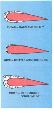
There are three types of structural icing clear, rime and mixed. They are shown in figure 1 and discussed in detail below.

2.4.1     Clear Ice

When an aircraft initially comes in contact with the liquid, there are some water droplets which stick at the point of contact. The remaining droplets flow over the surface of the aircraft which steadily freeze forming a smooth sheet of solid ice on the surface of the aircraft. This solid is the clear ice. However, this type of ice only occurs when the droplets of water, in rain or the cumuliform clouds, are large enough. The properties of clear ice include being hard, heavy and firm making it extremely difficult to remove, even with use of de-icing equipment. Hence, it can be seen why this type of ice would have a deep impact on aircraft aerodynamics are its properties significantly increase the overall weight of the aircraft which has a direct effect the lift and drag of the aircraft. Clear Ice also changes the shape of the aerofoil, again effecting the lift and drag characteristics of an aircraft. Typically, clear ice occurs between temperatures of 0 and -10 degree Celsius (Chapter 10 – ICING, 2017).

2.4.2     Rime Ice

Unlike clear ice, rime ice is formed when the water droplets are small. The remaining droplets, after the initial contact of the aircraft with liquid, freeze swiftly preventing the drops to spread. Rime ice has milky look to it as air is trapped between these frozen droplets. Compared to clear ice, rime ice is significantly lighter in weight, hardly having any effect on the weight of the aircraft. However, the rime ice makes the surface of the aerofoil rough and forms and irregular shape on the surface, which decreases the aerodynamic efficiency of the aerofoil. Hence, increasing drag and reducing lift. The properties of rime ice are that its brittle, making it easier to remove when compared to clear ice. Typically, rime ice occurs between temperatures of -15 and -20 degrees Celsius (Chapter 10 – ICING, 2017).

2.4.3     Mixed Ice

Mixed ice is a mixture of clear and rime ice, as suggested by the name. Mixed ice forms when different sized water droplets rapidly freeze when they come in contact with the surface of the aircraft. In comparison to rime and clear ice, mixed ice has the worse characteristics purely because of the increased roughness on the surface of the aircraft. Typically, mixed ice occurs between the temperatures of -10 and -15 degrees Celsius (Chapter 10 – ICING, 2017).

2.5      Similar Wind Tunnel Experiments

Broeren et al., 2011, undertook a study on different ice accretion on the leading of a wing. They performed a test in NASA’s Icing Research Tunnel (IRT) which is a is a “closed-return, refrigerated wind tunnel that contains a system of spray nozzles that are used to simulate in-flight icing cloud conditions”. The aerofoil used in their experiment was the NACA 23012. The test was performed for two different models, a sub-scaled wing model and a full-scaled wing model. The types of ice accretion they used was different to the ones in this study. However, the effects would be similar and can be compared with the results of this study. They used Horn ice simulation and Spanwise-Ridge ice simulation which is very similar to rime ice. They obtained data for pressure distribution across the aerofoil by adding pressure taps at various locations on the model. These taps record the pressure at that point for given flow and thus, a pressure distribution can be plotted. A similar pressure distribution is shown Chapter 5.2.

To summarise, their results can be used as benchmark to compare effects as their results are highly reliable. This is due to the fact that they used actual ice for simulation and in an iced wind tunnel which replicate real flight conditions.

2.6      Similar Numerical Simulation

A similar numerical simulation to the one performed in this project was undertake by Da-lin and Wei-jian, 2005. Their simulation emphasized on rime ice accretion process on an aerofoil. They incorporated a two-phase model of super-cooled droplets. This is a very useful model as this simulation provides an actual representation of rime ice accretion on the wing. Da-lin and Wei-jian, 2005, explain that “Incorporating the two-phase model of air-supercooled droplets in the Eulerian coordinate system, this technique is applied to simulate the process of the rime ice accretion (the droplets freeze at the instant impinging on the airfoil) on the NACA 0012 airfoil, and the ice profile after ice accretion is achieved successfully”. The reason these water droplets freeze at contact with the aerofoil is due to the temperature. A constant freezing temperature is maintained to allow these super-cooled droplets to freeze. The effects of ice are evaluated by plotting surface pressure distribution for clean and iced aerofoil. Similar, plot is generated for numerical results in this study shown and discussed in Chapter 6.2.1.

3         THEORECTICAL RESULTS

In this chapter, I will calculate the theoretical results of the NACA 0012, used at the wing tip of the Cessna 152 aircraft. The aim of his project is to investigate the aerodynamic performance and therefore it is essential to analyse the changes in the lift and drag forces of the aircraft. Therefore, I will be calculating the coefficient of lift and drag for the NACA 0012 aerofoil. However, it is quite challenging to calculate the lift coefficient theoretically as it is normally obtained using wind tunnel tests. But, it is possible to obtain 2D lift coefficient of the airfoil shape and then convert it to 3D, based on the span and chord of the wing. This can then be used as theoretical data to compare it with the experimental, wind tunnel, test. The drag can be calculated theoretically. I will be investigating the aerodynamic performance at three different Reynold’s Numbers 20000, 250000 and 30000. These correspond to velocities of 11.8 ms^-1, 14.8 ms^-1 and 17.8 ms^-1 respectively. These values are obtained using calculations shown below. The Reynolds number is given by:

Re= ρ*v*lμ

Equation 3‑1

Where,

• ρis the density of the air at sea level. This value is obtained from the International Standard Atmosphere (ISA).
• v is the velocity of the travelling air.
• lis the chord length of the wing.
• μis the dynamic viscosity at given condition (Sea Level for this project). This value is obtained to be 1.81E-5 from ISA

Rearranging Equation 3‑1 in terms of velocity would allow me to calculate the velocity.

v= Re*μρ*l= 200000*1.81×10-51.225*0.25= 11.8 ms-1

Equation 3‑2

Equation 3‑2 shows a sample calculation of velocity of 200000 Reynolds number. The same equation was used to obtain velocity for different Reynolds numbers.

I will be using the XFOIL v6.99, a Subsonic Airfoil Development Software, to obtain 2D lift coefficient and then convert it to 3D. XFOIL is obtained from Drela, 2017. The XFOIL Pressure distribution and command window of Reynold’s Number of 300000 is shown in APPENDIX A – XFOIL Pressure Distribution and Command Window for Reynold’s Number of 300000..

3.1      Reynolds Number of 200000

This section shows the lift and drag coefficients obtained from XFOIL v6.99. As mentioned earlier, these are two dimensional coefficients and therefore these will have to be converted to three dimensional to allows us to compare it with our experimental and numerical (CFD) results. The lift and drag coefficients will be obtained for three different Reynold’s Numbers. This would allow us to analyse the effects of ice on aerodynamic performance at different speeds. Hence, three different Reynolds Numbers were chosen.

3.1.1     Theoretical Lift Coefficient

Angle of Attack (degrees)	Cl 2D
-4	-0.5358
-2	-0.3084
0	0
2	0.3084
4	0.5357
6	0.6975
8	0.8494
10	1.0068
12	1.0993
14	0.9632
16	0.7085

Table 1 shows 2D coefficients obtained from XFOIL. These can now be converted into 3D. To do this, the two-dimensional lift-curve slope must be calculated. This is essentially the gradient of plot, lift coefficient against the angle of attack.

Table 1 2D Lift Coefficient for 200000 Reynold’s Number

The equations and calculations needed to obtain the theoretical lift coefficients are shown below. Equation 3‑3 shows the calculated lift curve slope for the data obtained from XFOIL shown in Table 1.

2D Lift Curve Slope= ΔY∆X= ΔClΔα = 0.9632–0.535814–4* 180°π= 4.77 radians-1

Equation 3‑3

This 2D lift curve slope can now be used to calculate the 3D lift curve slope by taking 3D effects into account. These effects include the Aspect Ratio (AR) and the Oswald Efficiency (e) of the wing. For an aspect ratio of less than 4, It can be calculated using Equation 3‑4 (Mh-aerotools.de, 2017).

3D Lift Curve Slope= 2D lift curve1+2D lift curveπ*AR*e2+2D lift curveπ*AR*e

Equation 3‑4

Where,

• AR is the Aspect Ratio of the Wing
• e is the Oswald Efficiency of the wing.

The aspect ratio is the ratio between the wing span (b) and the wing area (S). The model of the wing that I have manufactured, for this project, is scaled down by a factor of 18 from the actual wing span of Cessna 152. The wingspan of Cessna 152 is 33.4 inches which is approximately 10.2 metres and therefore my model is 0.575 m. The chord length of my wing is 0.25 m and therefore my wing planform area is 0.25*0.575 = 0.14375 m². These values were chosen to meet the requirements of the wind tunnel that was used to obtain experimental results for this project, this is discussed in further detail in chapter 5. The aspect ratio can be calculated using Equation 3‑5 shown below.

AR= b2S= 0.57520.14375=2.3

Equation 3‑5

Oswald efficiency factor is calculated using equation 3-4 (Sadraey, 2009).

e =1.781-0.0045AR0.68-0.64 =1.781-0.00452.40.68-0.64 =1.13

Equation 3‑6

Hence, substituting the values from Equation 3‑5 and Equation 3‑6 into Equation 3‑4, the 3D lift curve slope can be calculated.

3D Lift Curve Slope= 4.771+4.77π*2.3*1.132+4.77π*2.3*1.13=2.74 radian-1

This lift curve slope can be used to calculate the theoretical lift coefficient which can be used to for comparison. The 3D lift coefficient is given by substituting values from Table 1, Equation 3‑3 and Equation 3‑5 into Equation 3‑7 (Mh-aerotools.de, 2017).

CL= Cl3D lift curve2D lift Curve

Equation 3‑7

Where,

Clis the 2D lift coefficient obtained from XFOIL. A sample calculation for

α= -4°is shown below. The 2D lift coefficient (C_l) for

α= -4°is -0.5358, hence 3D lift coefficient (C_L) is

CL= Cl3D lift curve2D lift Curve= -0.53582.744.77= -0.307

 

 

 

 

 

 

Angle of Attack (Deg)	Cl 2D	Lift Curve 2D	Lift Curve 3D	CL 3D
-4	-0.5358	4.77	2.74	-0.3075
-2	-0.3084	4.77	2.74	-0.1770
0	0.0000	4.77	2.74	0.0000
2	0.3084	4.77	2.74	0.1770
4	0.5357	4.77	2.74	0.3074
6	0.6975	4.77	2.74	0.4003
8	0.8494	4.77	2.74	0.4874
10	1.0068	4.77	2.74	0.5778
12	1.0993	4.77	2.74	0.6308
14	0.9632	4.77	2.74	0.5527
16	0.7085	4.77	2.74	0.4066

Table 2shows all the calculated values for different angles of attack. This will data will be used as theoretical data for Reynolds number 20000 during analysis.

The above calculation can be performed for all angles of attack to obtain the theoretical lift coefficient.

3.1.2     Theoretical Drag Coefficient

The theoretical drag calculations are different to that of lift. Since I am only evaluating the aerodynamics of the wing of Cessna 152, I will only be calculating the drag of the wing. There are two different types of drag that combine to give the total drag of a given aircraft’s component. The two types of drag are parasitic drag and induced drag.

The parasitic drag is the zero lift drag of an aircraft. The parasitic drag is due to the skin friction of the aerofoil; thus, it is sometimes referred to as skin friction drag. All the different components of the aircraft such as wing, fuselage and tail contribute to the total parasitic drag. The parasitic drag varies at different flight conditions like cruise or landing. This is due to the fact and the parasitic drag is the function of MACH and Reynolds number and they both change at different conditions as the density and the speed vary. Hence, it is important to calculate the parasitic drag for all the three different Reynolds number that I have chosen.

Induced drag is the drag due to the lift produced by the wing. “The drag that results from the generation of a trailing vortex system downstream of a lifting surface with a finite aspect ratio. In another word, this type of drag is induced by the lift force” (Sadraey, 2009). Induced drag is a function of the wings aspect ratio and Oswald efficiency.

The total drag coefficient (

CD) of the wing is given by

CD= CDoW+ CDi

Equation 3‑8

Where,

• CDoWis the parasitic drag of the wing.
• CDiis the induced drag of the wing.

Angle of Attack (Deg)	CDoW
-4	0.01176
-2	0.01066
0	0.0102
2	0.01066
4	0.01176
6	0.01513
8	0.02076
10	0.02975
12	0.04416
14	0.11774
16	0.18817

The parasitic drag is obtained from XFOIL, similar to that of lift coefficient. Below is the table showing the values of parasitic drag obtained for different angles of attack.

Table 3 summaries the obtained drag values from XFOIL. These values correspond to Reynolds number of 200000. These contribute to the overall drag of the wing.

Table 3 Skin Friction Drag from XFOIL

The induced drag is given by

CDi= CL2π*AR*e

Equation 3‑9

Where,

• CLis the 3D coefficient of lift shown in Table 2.
• ARis the aspect ratio calculated in Equation 3‑5.
• eis the Oswald efficiency calculated in Equation 3‑6.

A calculation of induced and total drag for

α= -4°is shown below

CDi= CL2π*AR*e= -0.30752π*2.3*1.13=0.0116

The induced drag also changes with lift and therefore it is calculated for all the angles of attack as the lift changes with angles of attack. It is calculated using the same method shown  in the above equation using values for lift coefficient from Table 2 for different angles of attack.

Hence, substituting the values from Table 3 and Equation 3‑9 into Equation 3‑8 gives the value of the theoretical drag for

α= -4°.

CD= CDoW+ CDi=0.01176+0.0116=0.0233

The above calculation is repeated for different angles of attack and the theoretical value of drag is obtained. Table below shows all the calculated values of drag.

Angle of Attack (Deg)	CDoW	CDi	CD
-4	0.01176	0.0116	0.0233
-2	0.01066	0.0038	0.0145
0	0.0102	0.0000	0.0102
2	0.01066	0.0038	0.0145
4	0.01176	0.0116	0.0233
6	0.01513	0.0196	0.0348
8	0.02076	0.0291	0.0499
10	0.02975	0.0409	0.0706
12	0.04416	0.0487	0.0929
14	0.11774	0.0374	0.1552
16	0.18817	0.0202	0.2084

Table 4 Theoretical Drag Coefficient for Reynolds Number of 200000

Table 4 shows the theoretical drag coefficients that will be used for analysis.

3.2      Reynolds Number of 250000

The theoretical for Reynold’s number of 250000 are calculated in the same way as shown in section 3.1 of this chapter. Equations from section 3.1.1 and 3.1.2 of this chapter were used to calculate the theoretical lift and drag coefficients for this Reynolds number. The only difference here would be that the speed changes due to Reynolds number. Below is the summary table showing both the lift and drag coefficients.

Angle of Attack (Deg)	Cl 2D	2D Lift Curve	3D lift Curve	CL 3D	CDoW	CDi	CD
-4	-0.5371	5.12	2.83	-0.2972	0.01105	0.0108	0.0219
-2	-0.2664	5.12	2.83	-0.1474	0.00959	0.0027	0.0123
0	0.0000	5.12	2.83	0.0000	0.00863	0.0000	0.0086
2	0.2664	5.12	2.83	0.1474	0.00959	0.0027	0.0123
4	0.5370	5.12	2.83	0.2972	0.01105	0.0108	0.0219
6	0.7029	5.12	2.83	0.3890	0.01412	0.0185	0.0326
8	0.8563	5.12	2.83	0.4738	0.01899	0.0275	0.0465
10	1.0104	5.12	2.83	0.5591	0.02663	0.0383	0.0649
12	1.1260	5.12	2.83	0.6231	0.0378	0.0475	0.0853
14	1.0709	5.12	2.83	0.5926	0.062	0.0430	0.1050
16	0.7128	5.12	2.83	0.3944	0.18616	0.0191	0.2052

Table 5 Theoretical Lift and Drag Coefficients for Re 250000

3.3      Reynolds Number of 300000

The theoretical calculations for this Reynolds are, again, calculated using methods and equations shown in section  3.1.1 and 3.1.2 of this chapter. Hence, they have not been repeated here and a summary table is shown below.

Angle of Attack (Deg)	Cl 2D	2D Lift Curve	3D lift Curve	CL 3D	CDoW	CDi	CD
-4	-0.540	5.137	2.837	-0.298	0.01056	0.0109	0.0214
-2	-0.238	5.137	2.837	-0.131	0.00875	0.0021	0.0109
0	0.000	5.137	2.837	0.000	0.00768	0.0000	0.0077
2	0.238	5.137	2.837	0.132	0.00875	0.0021	0.0109
4	0.540	5.137	2.837	0.298	0.01056	0.0109	0.0214
6	0.708	5.137	2.837	0.391	0.01337	0.0187	0.0321
8	0.863	5.137	2.837	0.477	0.01785	0.0278	0.0457
10	1.013	5.137	2.837	0.559	0.02398	0.0383	0.0623
12	1.125	5.137	2.837	0.621	0.03402	0.0473	0.0813
14	1.074	5.137	2.837	0.593	0.05881	0.0431	0.1019
16	0.702	5.137	2.837	0.388	0.18518	0.0184	0.2036

4         EXPERIMENTAL RESULTS

This chapter explains the process of obtaining my experimental results. The aircraft I have chosen is Cessna 152 and so I will be using its aerofoil to produce my model of the wing. As mentioned before, I will be assuming a constant aerofoil shape, NACA 0012, across the span wing to reduce the complexity of the project. Figure 2 shows the aerofoil shape of NACA 0012.

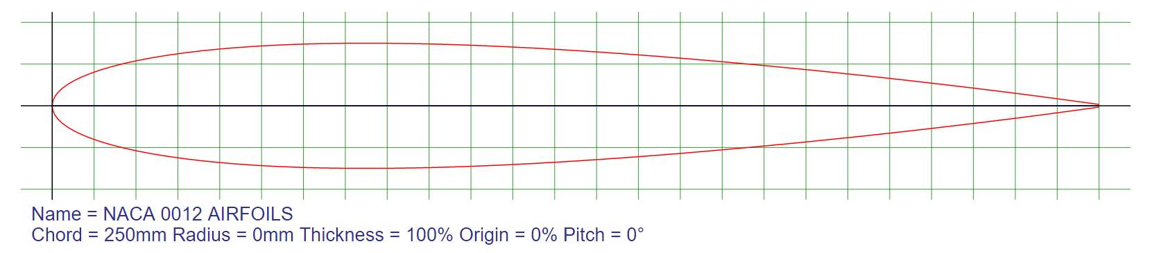
Figure 2 NACA 0012 Aerofoil (“NACA 0012 AIRFOILS (N0012-Il)”)

To obtain the experimental results, I will be performing the wind tunnel test with different configurations. These configurations are clean wing, rime iced wing, clear iced wing and mixed ice wing (Section 2.3). This is undertaken to effectively analyse the effects of different types of ice on aerodynamic performance of an aircraft. Hence, I will be casting these different types of ice on my wing to evaluate their effects. However, it is very difficult to apply actual ice to the wing due to its properties. Therefore, I will be an alternate material that can replicate ice and its effects. The choice of material is discussed in section 4.1.3 of this chapter.

4.1      Wing Model

Initially, I had decided that I would develop the wing model for my wind tunnel test using a 3D printer which uses plastic as a material. However, I will now be using wood as my primary material for my model and physically manufacture the model and not use a 3D printer. I made this decision after comparing different approaches and taking advices from different technicians at the university and it was concluded that for the purpose of this project, physically manufacturing would be appropriate especially with the wind tunnel requirements (discussed in section 4.2). It is also a lot cheaper to take this approach than to use a 3D printer as 3D printing is very expensive. The process of manufacturing my wing is discussed in this section.

4.1.1     CAD Model

Firstly, a 3D model of the wing was developed using CATIA V5, a powerful 3D modelling software widely used in industry. The wing was modelled by importing the coordinates of the aerofoil to produce a precise shape of the aerofoil (The coordinates of the aerofoil are shown in APPENDIX B – NACA 0012 Aerofoil Coordinates. Figure 3 shows the 3D model of my wing.

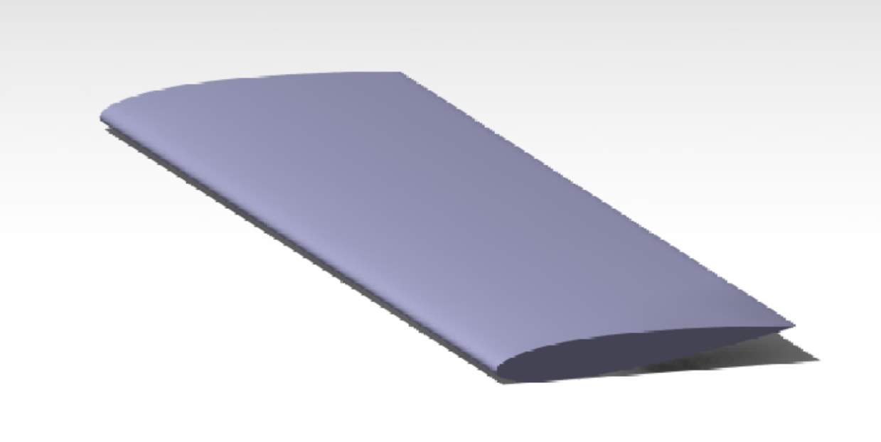
Figure 3 CATIA Model of the Wing

4.1.2     Manufacturing Process

The wing was manufactured using Balsa wood, this was done by consulting technicians at the university and their approval. The first step of developing the wing was creating the inner ribs of the wings. The ribs created using a Laser Cutting machine available at the University of Hertfordshire. This was done by importing a drawing of the rib, obtained from CATIA V5 using the NACA 0012 coordinates.

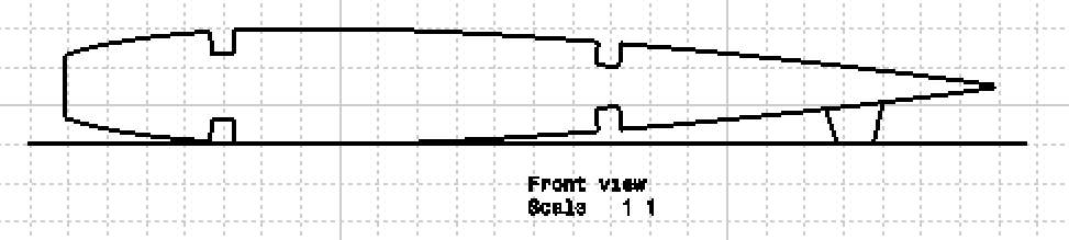
Figure 4 Drawing of the Rib

Figure 4 shows the CATIA drawing of the rib which was imported in the laser cutting machine to cut the wood in the shape of the rib. The four boxed pockets in the above figure represent the space where the spars would be connected. A total number of 10 spars were chosen across the span of the wing and the Balsa wood used for the ribs had a thickness of 10mm. The horizontal distance between the two spars was chosen two be 100mm and the distance between the trailing edge of aerofoil and the trailing edge spar was also 100mm. These distances were chosen because the wood skin that will be used to cover the ribs and spars and obtain the shape of the wing has width of 100 mm. Hence, it was important to place the spars as they were to allow for the skin to glue in place since super glue was used for the assembly of the model. The spars were 5mm square rod.

Once the ribs were laser cut, the wing was assembled. The assembly process involved attaching the ribs with the spars using super glue and then placing the skin to complete the wing.  The final process was to sand the entire wing thoroughly using sand paper to avoid any roughness on the surface and ensure it is smooth. This is very important as the data obtain as a result of a rough surface is not very accurate. Hence, a smooth surface would ensure that there is no interference in the flow during the wind tunnel test.