Does Financial Development Stimulate Investment Financing?

Topic: Does financial development stimulate firms’ investment financing? A study in Vietnam

Chapter 1: Introduction

Chapter 2: Literature review

2.1 Sources of firms’ financing

For the purpose of this paper, investment refers to capital expenditure (Capex), which is measured by spending on plant, property and equipment. Basically, firm’s investment is financed by using two sources of finance: internal finance and external finance. Internal finance, i.e. self-financing, may consist of four main components: past profits which are not distributed to shareholders; additional capital from the owners; depreciation and amortization. Besides taking the advantages from itself when collecting internal sources for investment, firm might also use external source from loans of banks and other financial institutions or issue of new equity. This section is divided into two subsections: the former covers internal financing and the later external financing.

2.1.1 External financing

2.1.2 Internal financing

There is a vast literature documenting the state that the greatest source of investment financing comes from internal sources. According to Sweezy (1968), the firm’s profits growth mainly contributes to the capital accumulation gain for the purpose of production expansion. Moreover, Mayer (1990) used US firms’ data from 1970-1985 to provide an empirical evidence that in this case, firms mostly rely upon internal sources. The result is similar to the study of British firms of chemical and electrical engineering industries from 1949-1984 that bank loans and bond securities do not play a significant role to fixed investment financing (see Table 1 ). However, he also argued that bank loans which are considered as the main source of external finance mostly contribute to firms’ working capital.

Using the same data of two industries in UK but with the different approach, Mayer (1990) examined the variation of capital structure according to the firm size. Table 2 points out that large firms seem to require more on internal financing in comparison with external financing.

Corbett and Jenkinson (1997) provide another evidence to support the Mayer’s findings by analyzing the source of finance of three developed countries including Germany, the US and the UK from 1970-1994. The study shows that in the period 1970-1994, the firms in these countries mostly rely on the internal source of finance with the average proportion of the internal finance and total fixed investment of 78.9 percent in Germany, 93.3 percent in the UK and 96.1 percent in the US. These are stories in developed countries.

What happens in the countries with the state control over financial system? In these countries, state development banks and other state owned banks follow low interest rate policies to stimulate investment (Singh, 1998), especially in the early stage of development. The poof indicates that the most fundamental source of finance for fixed investment comes internal finance; however the share of long-term bank loans were still high compare to the rate in developed countries mentioned above. Choosing Japan before becoming a developed country in 1990’s as the case of state control over financial system, Tsuru (1993) figured out that the share of internal financing over gross manufacturing investment accounted for 60 percent in the late 1950s, increasing to 75 percent in the late 1970’s and around 100 percent in the late 1980’s. The long-term bank loans covered the rest of investment financing, and had continued declining from 1950’s. China is a typical example for the country with the financial system regulated by the government. According to Fisher (2013), the Chinese government plays a central role in the financial system. It is demonstrated by the fact that the proportion of the total assets of state-owned commercial banks and development banks to total banks’ asset accounts for roughly 60 percent. Mlachila and Takebe (2011) argued that due to the government regulation, these banks can lend lower interest rate to firms, especially with state-own enterprises investing in construction, logistic and heavy manufacturing.

Chapter 3: Model specification and hypotheses development

This chapter contains three main parts. The first part presents the theoretical framework to model investment. As mentioned in the previous part, so-called Euler investment equation approach as well as how to use it to test for the presence of financing constraints would be presented here. The second part specifies the model which is expected to test the impact of financial development on firm investment. Hypotheses for the model would be also displayed in the last.

3.1 Modeling investment

3.1.1 Euler equation approach

After the first introduce of Abel (1980), the investment Euler equation approach was widely used by many authors (White, 1992; Hubbard, Krashyap & White, 1995; Bond & Meghir, 1994; Harris, Schiantarelli & Siregar, 1994, Gilchrist & Himmelberg, 1999; Love, 2003; Laeven, 2003; Forbes, 2007, K.S.Chan et al., 2012). The equation is acquired after reorganizing first order conditions when solving the maximizing firm’s value problem.

In this paper, the investment model based on Euler equation approach closely follows models in previous studies, especially Laeven (2003) and Bond & Meghir (1994). To construct the model, each firm is assumed to maximize its present value. The firm value is the sum of the expected discounted value of dividends subject to the capital accumulation and external financing constraint. 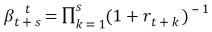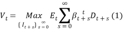Let be the firm value at time t, the the dividend paid to shareholder at time t, and the one period discount factor, and Then, the function of firm value at time t is presented in (1) in which E(.) is the expectations operational on time t information. Let = denote the profit function taking as the beginning of period capital stock at time t, ; the vector of variable inputs at time t, and the firm investment at time t, . The profit function is assumed to be concave and bounded according to Gilchrist (1999). 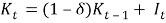With the depreciation rate and the investment expenditure at time t, , the capital stock accumulation follows this formula: 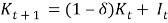. Finally, let be the financial liabilities. Under the assumption that the marginal source of external finance is debt and that risk neutral debt holders tend to require an external premium, . This premium is expected to be increasing in the amount borrowed to offset the raised costs due to information asymmetry problems. Following Gilchrist (1999) and Laeven (2003), the gross required rate of return on debt is assumed to be equal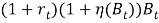, where is the risk-free rate of return.

To ensure that the only debt is the firm’s marginal source of finance, a non-negativity constraint on dividends is introduced. It also means that shareholders favor dividends paid out instead of retention. For all of the above, the manager’s problem of maximizing firm’s value is presented as follow:

Subject to:

(2)

(3)

(4)

Let λ_t be the Lagrange multiplier for the non-negativity constraint on dividends in equation (4) to recognize the effect of financial friction. λ_t is the shadow cost of paying negatives dividends, i.e. issuing new equity. Therefore, in economic meaning, it can be defined as the shadow cost of internally generated funds.

Substituting in (2) into (1) and using (3) to eliminate in the profit function, the Lagrangian function is constructed as:

(5)

Taking the first order condition for K_t :

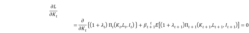
(6)

Because =>

So, (7). Substituting (7) into (6):

Rearranging the equation below to obtain the Euler equation:

(8)